Canonical Quantum Phase Estimation AlgorithmDeterministicQPE

Quantum phase estimation (QPE) is a quantum algorithm used to estimate the phase \(\phi \in [0, 1)\) of a given unitary operator \(U\) and eigenstate \(|\phi\rangle\) satisfying

(23)\[U|\phi\rangle = e^{i2\pi\phi} |\phi\rangle .\]

QPE based on the quantum Fourier transform (QFT) [11, 12, 13, 14] is referred to as canonical QPE. QFT can be considered to be a quantum analog to the discrete Fourier transform, and is expressed as:

(24)\[|j\rangle \longrightarrow \frac{1}{\sqrt{N}} \sum_{k} \exp\left({i\frac{2\pi jk}{N}}\right) |k\rangle\]

where \(N\) is the total number of states. This general expression can be rewritten with \(n\) qubits as

(25)\[|j_{1}\cdots j_{n}\rangle \longrightarrow \frac{1}{\sqrt{2^{n}}} \left( |0\rangle + e^{i2\pi 0.j_{n}}|1\rangle \right) \otimes \cdots \otimes \left( |0\rangle + e^{i2\pi 0.j_{1}j_{2}\cdots j_{n}}|1\rangle \right)\]

where the binary fraction is represented as \(0.j_{1}\cdots j_{n} = \sum_{k=1}^{n} j_{k} 2^{-k}\). The basic idea of the canonical QPE is to compute the right-hand side of QFT using Eq. (23) and estimate the phase factor as a bit string by the inverse QFT.

To do this, canonical QPE uses two quantum registers. The first register contains \(n\) qubits initially in the state \(|+\rangle = \frac{1}{\sqrt{2}}(|0\rangle + |1\rangle)\). The choice of \(n\) depends on the precision of the estimate of \(\phi\) we wish to reach. The second register is initialized in the state \(|\phi\rangle\), and contains as many qubits as is necessary to represent \(|\phi\rangle\).

We compute the right-hand side of (25) using the phase kickback technique:

(26)\[|+\rangle \otimes |\phi\rangle \xrightarrow{\mathrm{ctrl-}U^{2^{k-1}}} \frac{1}{\sqrt{2}}\left( |0\rangle + e^{i2\pi 0.\phi_{n-k+1}\phi_{n-k}\cdots \phi_{n}} |1\rangle \right) \otimes |\phi\rangle\]

The example of the canonical QPE circuit is shown in Fig. 4.

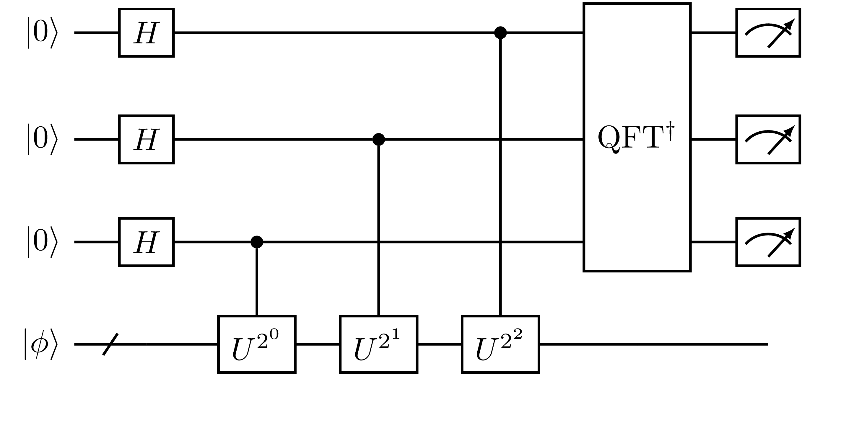
Fig. 4 Example of the canonical QPE circuit with three ancilla qubits.

In chemistry, QPE is most often proposed within the context of calculating molecular energies. For this purpose, we set the unitary to the time evolution operator \(U(t) = e^{-iHt}\), where \(H\) is the Hamiltonian describing the system. \(t \in \mathbb{R}\) is a parameter. Then, the eigenstate energy is obtained as \(E = -2\pi\phi / t\). The initial state is chosen to be some trial electronic wavefunction \(|\Phi\rangle\), such as the Hartree-Fock state. The “quality” of the initial state is an important factor to obtain the target phase value efficiently, as the probability of obtaining \(\phi\) is dependent on the overlap \(\langle \phi | \Phi \rangle\). One can also use an ansatz that has been optimized, such as by VQE, which may lead to a reduction in the overall computational time.

AlgorithmDeterministicQPE may be used for performing the canonical QPE algorithm. The phase estimation circuit requires subcircuits which perform repeated sequences of the unitary evolution operator controlled upon the ancilla qubits. We refer to one of these sequences as \(\mathrm{ctrl-}U\). Here, to prepare \(\mathrm{ctrl-}U\) from the molecular Hamiltonian \(H\), we follow the same steps as those for AlgorithmVQE.

from inquanto.express import get_system
from inquanto.mappings import QubitMappingJordanWigner

target_data = "h2_sto3g.h5"
fermion_hamiltonian, fermion_fock_space, fermion_state = get_system(target_data)
mapping = QubitMappingJordanWigner()
qubit_hamiltonian = mapping.operator_map(fermion_hamiltonian)

Currently, InQuanto supports the Suzuki-Trotter decomposition to construct the \(\mathrm{ctrl-}U\) circuit (shown in the cell below). Several methods have been proposed in the literature with different asymptotic scaling, such as quantum signal processing. [17]

# The parameter `t` that is physically recognized as the time period in atomic units.
# In this case this constant is chosen to demonstrate the impact on phase discretization
time = 0.40723

# Generate a list of qubit operators as exponents to be trotterized.
qubit_operator_list = qubit_hamiltonian.trotterize(trotter_number=1, constant=time)

The initial state \(|\Phi\rangle\) is provided as a non-symbolic ansatz. The example below uses a modestly optimized UCCSD ansatz for the state preparation circuit.

from inquanto.ansatzes import FermionSpaceAnsatzUCCSD

# Preliminary calculated parameters.
ansatz_parameters = {"d0": -0.10723347230091586,"s0": 0.0, "s1": 0.0}

# Generate a non-symbolic ansatz.
ansatz = FermionSpaceAnsatzUCCSD(fermion_fock_space, fermion_state, mapping)
state_prep = ansatz.subs(ansatz_parameters)

An AlgorithmDeterministicQPE instance is then constructed from this ansatz and the list of qubit operators.

from inquanto.algorithms import AlgorithmDeterministicQPE

algorithm = AlgorithmDeterministicQPE(
    state_prep,
    qubit_operator_list,
)

Then, we build a protocol to construct a canonical QPE circuit. n_rounds specifies the number of ancilla qubits of the first quantum register, which determines the precision of the computation. Together with the four qubit representation hydrogen molecule state the circuits have a total of eight qubits.

from pytket.extensions.qiskit import AerBackend
from inquanto.protocols import CanonicalPhaseEstimation, MeasurementPluralityPhaseEstimator

# Choose the backend.
backend = AerBackend()

# Set the number of rounds (ancilla qubits of the first quantum register)
n_rounds, n_shots = 4, 100

# Chose the protocol to specify how the circuit is handled.
protocol = CanonicalPhaseEstimation(
    backend=backend,
    n_rounds=n_rounds,
    n_shots=n_shots,
)
# Optional phase estimator, converts experimental results to a phase for later evaluation
estimator = MeasurementPluralityPhaseEstimator()

# Build the algorithm to get it ready for experiments.
algorithm.build(
    protocol=protocol,
    phase_calculation_protocol=estimator,
);

Now the circuit is run by algorithm.run() to produce the final results. The algorithm.final_energy() returns the energy estimate.

# Run the protocol.
algorithm.run()

# Display the final results.
energy = algorithm.final_energy(time=time, phase_estimator_protocol=estimator)
print(f"energy estimate  = {energy:8.4f} hartree")

# Store the experiment results for later plotting
counts_canonical = estimator.generate_report()["raw_counts"]

energy estimate  =  -1.2278 hartree

Sin-state QPE

In the previous section, the ancilla register of \(n\) qubits was prepared in the \(|+\rangle\) state

(27)\[|+\rangle^{\bigotimes n} = \frac{1}{\sqrt{2^m}} \sum_{k}^{2^m-1} |k\rangle,\]

which allowed us to prepare the QFT of the initial state \(|\phi\rangle\). This ancilla state preparation provides maximum phase accuracy in the noiseless case, but for fault-tolerant applications it is more optimal to prepare a sine state. [18]

(28)\[|\text{sin}\rangle = \sqrt{\frac{2}{2^m+1}} \sum_{k=0}^{2^m-1} \sin{\left(\frac{k+1}{2^m+1}\pi\right)} |k\rangle.\]

This has been shown to optimize the Holevo variance of the estimator \(C\), [19] which can be interpreted as minimizing the distance between the true phase \(\theta\) and a set of measured estimate \(\hat{\theta}\) values.

(29)\[C(\theta,\hat{\theta}) = 4\sin^2{ \frac{\hat{\theta} - \theta}{2} }.\]

The use of this estimator shows that we are now considering the measurement data variance and not just its mean value for estimating the phase. In the presence of noise, the non-uniform superposition \(|\text{sin}\rangle\) in Eq. (28) ensures that all the measurement results are distributed closer to the mean value and the probability density tails are diminished. [19] This variant of QPE is referred to as sin-state QPE. [18]

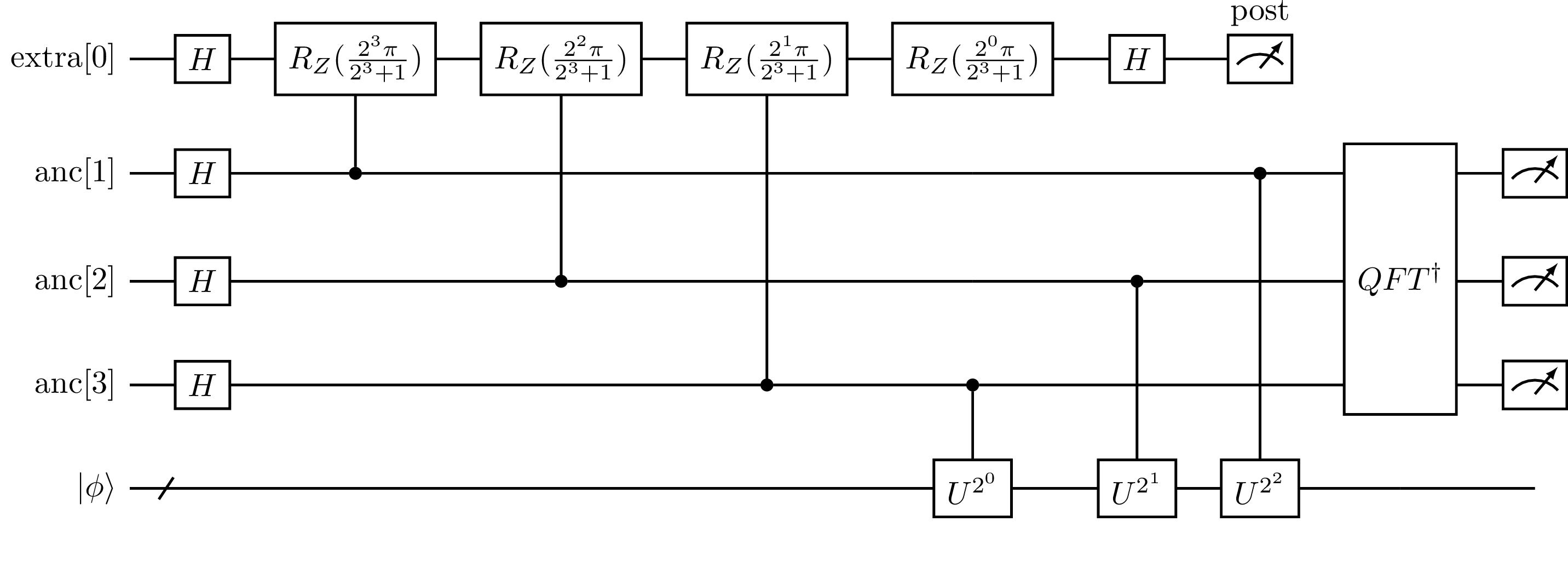
An example of a sin-state QPE circuit is shown below. It resembles the Canonical QPE circuit, but there is additional state preparation on the ancilla register. Furthermore, preparing the \(|\text{sin}\rangle\) state requires an additional ancilla qubit (shown at the top of the circuit), which is not used for the ctrl-U operations. In order to perform this state preparation, a post-selection on the extra ancilla qubit is needed.

Performing sin-state QPE in InQuanto is possible using AlgorithmDeterministicQPE, just like for the canonical case. However, the extra ancilla qubit requires the use of a SinStatePhaseEstimation protocol and the post-selection is performed using SinStatePhaseEstimator.

from inquanto.protocols import SinStatePhaseEstimation, SinStatePhaseEstimator

# Choose sin-state protocol to handle circuits
protocol_sin_state = SinStatePhaseEstimation(
    backend=backend,
    n_rounds=n_rounds,
    n_shots=n_shots,
)
# Choose sin-state estimator to post-select and evaluate final energy
estimator_sin_state = SinStatePhaseEstimator()

# Build the algorithm again with the sin-state protocol
algorithm.build(
    protocol=protocol_sin_state,
    phase_calculation_protocol=estimator_sin_state,
)

<inquanto.algorithms.phase_estimation._algorithm_phase_estimation.AlgorithmDeterministicQPE at 0x7f29577ca550>

The sin-state QPE protocol and estimator need to be included in the algorithm build() method and the final_energy() algorithm call needs to include the estimator as well.

# Run the algorithm again
algorithm.run()

# Display the final results.
energy_sin_state = algorithm.final_energy(
    time=time,
    phase_estimator_protocol=estimator_sin_state
)
print(f"energy estimate  = {energy_sin_state:8.4f} hartree")

energy estimate  =  -1.2278 hartree

To better understand the impact of sin-state QPE, we can plot the measurement results. The code below shows how to first retrieve the results from experiment, then process and plot them.

from pytket.utils import probs_from_counts
import numpy as np
from matplotlib import rcParams
import matplotlib.pyplot as plt

# Retrieve measurement results
counts_sin_state = estimator_sin_state.generate_report()["post_selected_counts"]

# Get the binary fractions from the ancilla register
def parse_bin(tup):
    return int("".join([str(x) for x in tup]), 2) / 2 ** len(tup)

# Process the experiment results
def process_probs(probs):
    energies = np.array([-2 * parse_bin(bi) / time for bi, count in probs.items()])
    results = np.array([p for bi, p in probs.items()])
    indexes = np.argsort(energies)
    return energies[indexes], results[indexes]

energies_canonical, results_canonical = process_probs(probs_from_counts(counts_canonical))
energies_sin_state, results_sin_state = process_probs(probs_from_counts(counts_sin_state))

# Plot the results
def plot_results(energies, results, title = "", axs = None):
    energy_ticks = ['{:.3f}'.format(x) for x in energies]
    axs.bar(energy_ticks, results)
    axs.set_xlabel("Energy")
    axs.set_ylabel("Probability")
    axs.tick_params(labelrotation=45)
    axs.set_title(title)

rcParams.update({'figure.autolayout': True})
fig, axs = plt.subplots(1, 2, figsize=(11,6))
plot_results(energies_canonical, results_canonical, f"Canonical QPE", axs[0])
plot_results(energies_sin_state, results_sin_state, f"Sin-state QPE", axs[1])
fig.suptitle(f"{target_data}, nr={n_rounds}, ns={n_shots}")
plt.show()

The final figure shows a comparison of canonical and sin-state QPE results for the h2_Sto3g system for 4 rounds and 100 shots. The initial state \(|\phi\rangle\) is prepared as a GS of the VQE calculation. It is apparent how sin-state QPE produces measurement peaks closer to the mean with no significant tails, which are visible for the canonical case.